Dimension Reduction with Principal Component Analysis

PCA is one of the most popular techniques for dimensionality reduction. If you have no idea what I mean by dimensionality reduction, check out part 1 of this topic. In this article, we’ll explore PCA with a more applied approach rather than mathematical and we’ll keep certain details in a blackbox for future discussions.

What is PCA? PCA is an algorithm that transforms a dataset to lower dimensional dataset. The keyword here is transform which is different from feature selection that I’ve talked about in part 1. The difference being that features are not removed from the dataset but instead the dataset itself is transformed. Simple hypothetical example:

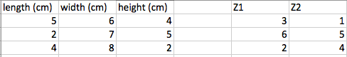
We have on the left the original dataset comprising of length, width, and height in centimetres. If we were to apply PCA to reduce this down to two dimensional dataset, we would get something like the right where we have two features, let say, Z1 and Z2. Z1 and Z2 is not produced from removing one of the features but instead all three features (L, W, H) are transformed and Z1 and Z2 does not represent the same measurements (cm) anymore.

The goal of this algorithm is to reduce the dimensions of the dataset while retaining majority of the information, meaning maximizing the amount of variance kept. Another way of interpreting this is that the algorithm looks for vector(s) when projecting the data that minimizes the overall projection error. Lets take a look at what this means:

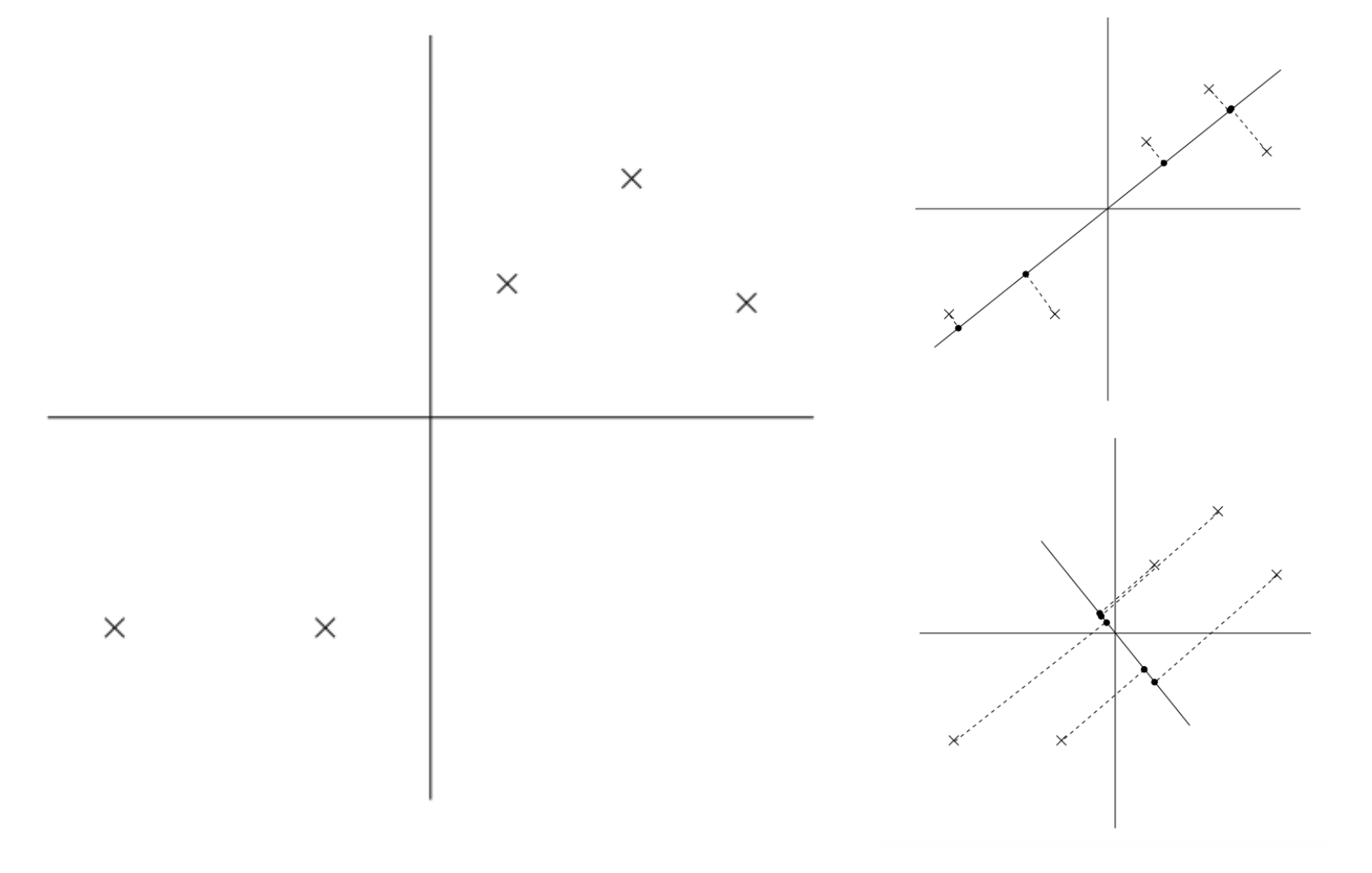
On the left we couple data points in 2D space that we hope to use PCA to reduce down to a one dimension vector. On the top right, we project the data onto the solid line. The dotted lines from the data point to the solid line is what we call the projection error. On the bottom right is another way of projecting the data onto another line. It is evident that the projection error of the bottom right graph is much bigger than the projection error of the top right. What is not as evident is that the variance of the projected data points on the line is much bigger for the top right graph vs. the bottom right. Whether it is to minimize projection error or maximize variance, PCA’s goal is to retain as much information about the dataset as possible.

For this reason, one important step before applying this algorithm is to perform normalization on the mean and variance for each feature and scaling on the range. A feature (before scaling) with a disproportionately large variance will be tend to be favoured in PCA because to the algorithm this feature explains majority of the variance in the original dataset.

Now that you have a high level conceptual understanding of PCA, checkout the notebook belong on practical examples of how to apply PCA with sci-kit learn! I will illustrate two examples, one to highlight visually the results of PCA on a simple 2D & 3D dataset and another applying PCA on a high dimensional dataset. For the high dimensional datset, I will use the same dataset from Kaggle about food nutrients that I’ve used previously.

https://www.kaggle.com/openfoodfacts/world-food-facts This data set has 134754 rows and 161 columns. One row per food product.

import pandas as pd
import numpy as np
from sklearn import datasets
from sklearn.decomposition import PCA
import matplotlib.pyplot as plt
%matplotlib inline
from sklearn import preprocessing

Defined # of Principal Components

We use the iris dataset from sklearn to demonstrate visually how to apply PCA on a 2D dataset and reduce to 1D and a 3D dataset into 2D.

iris = datasets.load_iris()

Before applying PCA, we need to normalize our data to mean of 0 and unit variance. We can use the scale function in the preprocessing module from sklearn.

X_2d = iris.data[:, :2] 
X_2d_scale = preprocessing.scale(X_2d)
print "Mean: " + str(X_2d_scale.mean(axis=0)).strip('[]')
print "Standard Deviation: " + str(X_2d_scale.std(axis=0)).strip('[]')

Mean:  -1.69031455e-15  -1.63702385e-15
Standard Deviation:  1.  1.

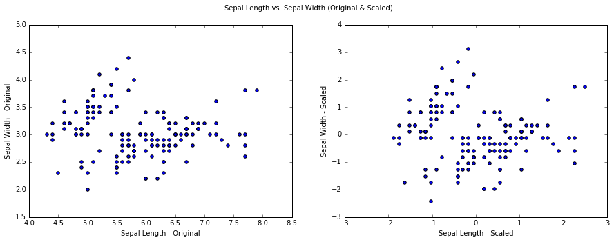
Plotting the original and scaled data set. The two plot looks very similar because the range and variance of Sepal Length and Sepal Width are naturally similar.

fig = plt.figure()
fig.set_size_inches(15, 5)
ax1= fig.add_subplot(121)
ax1.scatter(X_2d[:, 0], X_2d[:, 1])
ax1.set_xlabel('Sepal Length - Original')
ax1.set_ylabel('Sepal Width - Original')
ax2= fig.add_subplot(122)
ax2.scatter(X_2d_scale[:,0], X_2d_scale[:,1])
ax2.set_xlabel('Sepal Length - Scaled')
ax2.set_ylabel('Sepal Width - Scaled')
fig.suptitle('Sepal Length vs. Sepal Width (Original & Scaled)')

We want to reduce this dataset from 2D to 1D, using the PCA module from sklearn we specify to keep 1 component.

pca = PCA(n_components = 1)
pca_2d = pca.fit_transform(X_2d)

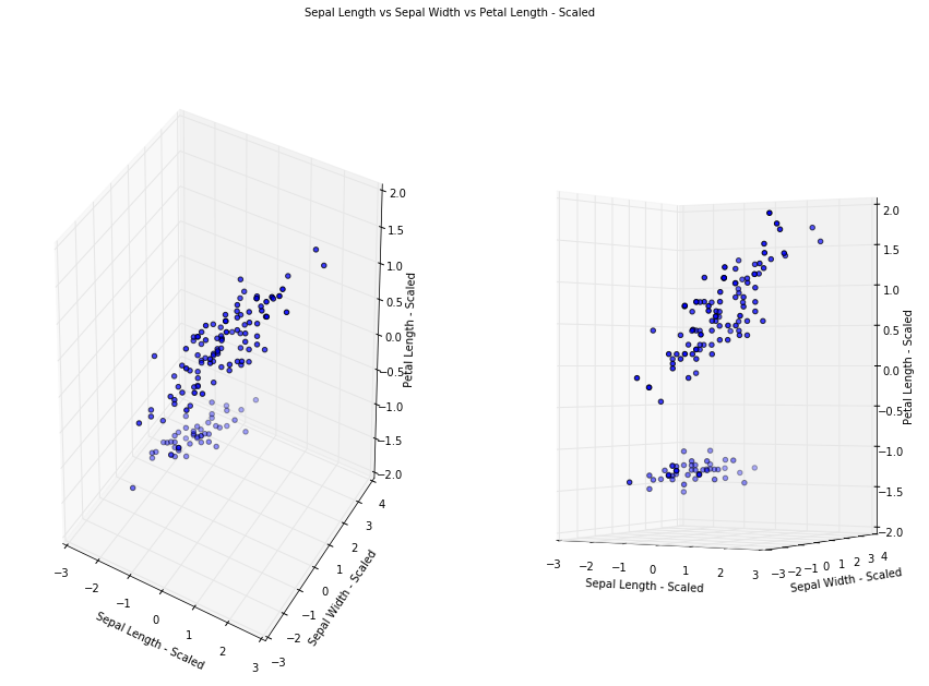
To demonstrate more visually the results of PCA, lets take a look at reducing 3D dataset to 2D. Like previously, we first normalize our dataset

X_3d = iris.data[:, :3] 
X_3d_scale = preprocessing.scale(X_3d)
print "Mean: " + str(X_3d_scale.mean(axis=0)).strip('[]')
print "Standard Deviation: " + str(X_3d_scale.std(axis=0)).strip('[]')

Mean:  -1.69031455e-15  -1.63702385e-15  -1.48251781e-15
Standard Deviation:  1.  1.  1.

from mpl_toolkits.mplot3d import Axes3D

fig = plt.figure()
fig.set_size_inches(15, 10)
ax1 = fig.add_subplot(121, projection='3d')
ax1.scatter(X_3d_scale[:, 0], X_3d_scale[:, 1], X_3d_scale[:, 2])
ax1.set_xlabel('Sepal Length - Scaled')
ax1.set_ylabel('Sepal Width - Scaled')
ax1.set_zlabel('Petal Length - Scaled')
ax2 = fig.add_subplot(122, projection='3d')
ax2.scatter(X_3d_scale[:, 0], X_3d_scale[:, 1], X_3d_scale[:, 2])
ax2.view_init(elev=0)
ax2.set_xlabel('Sepal Length - Scaled')
ax2.set_ylabel('Sepal Width - Scaled')
ax2.set_zlabel('Petal Length - Scaled')
fig.suptitle('Sepal Length vs Sepal Width vs Petal Length - Scaled')

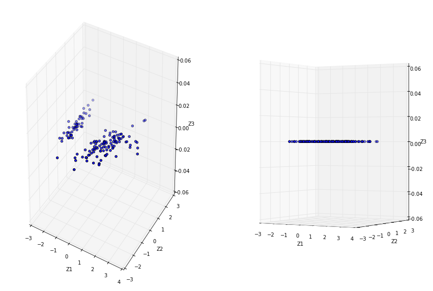
Specify to keep 2 principal components. After PCA, our dataset no longer represent Sepal Width, Sepal Length and Petal Length as PCA has transformed and projected our dataset into an arbitrary space, let say Z1, Z2, Z3

pca = PCA(n_components = 2)
pca_3d = pca.fit_transform(X_3d_scale)

fig = plt.figure()
fig.set_size_inches(15, 10)
ax1= fig.add_subplot(121, projection='3d')
ax1.scatter(pca_3d[:, 0], pca_3d[:, 1], 0)
ax1.set_xlabel('Z1')
ax1.set_ylabel('Z2')
ax1.set_zlabel('Z3')
ax2= fig.add_subplot(122, projection='3d')
ax2.scatter(pca_3d[:, 0], pca_3d[:, 1], 0)
ax2.view_init(elev=0)
ax2.set_xlabel('Z1')
ax2.set_ylabel('Z2')
ax2.set_zlabel('Z3')

Solving For Number Of Principal Components

Whats powerful about sklearn is that the same modules we used previously for PCA, under the circumstances that we don’t know the number of principal components prior to applying the reduction, can be used to solve for the number of principal components required to keep a certain % of variance within the dataset. Typically we want to retain 90%, 95% or 99% of the variance but depends on use case.

Lets use the same iris data as an example first then the food nutrient dataset from Kaggle.

iris_3d = X_3d_scale

To find the number of principal components, in the same PCA function, we define n_components to be 0 < n_components < 1 which is the % of variance that we want to keep in the dataset and we specify svd_solver == ‘full’. Lets start with 95% then 30% and see what happens

p_95 = PCA(n_components = 0.95, svd_solver='full')

p_95.fit(iris_3d)

PCA(copy=True, iterated_power='auto', n_components=0.95, random_state=None,
  svd_solver='full', tol=0.0, whiten=False)

print "We see that to keep 95% of the variance in the original dataset, we can reduce the dataset into 2D \n"
print "The number of components :" + str(p_95.n_components_)
print "The % of variance explained by each component: " + str(p_95.explained_variance_ratio_)

We see that to keep 95% of the variance in the original dataset, we can reduce the dataset into 2D 

The number of components :2
The % of variance explained by each component: [ 0.67127544  0.30494357]

p_30 = PCA(n_components = 0.30, svd_solver='full')

p_30.fit(iris_3d)

PCA(copy=True, iterated_power='auto', n_components=0.3, random_state=None,
  svd_solver='full', tol=0.0, whiten=False)

print "We see that to keep only 30% of the variance in the original dataset, we can reduce the dataset into 1D \n"
print "The number of components :" + str(p_30.n_components_)
print "The % of variance explained by each component: " + str(p_30.explained_variance_ratio_)

We see that to keep only 30% of the variance in the original dataset, we can reduce the dataset into 1D 

The number of components :1
The % of variance explained by each component: [ 0.67127544]

Applying PCA on food nutrient dataset from Kaggle

If you haven’t already, check out part 1 of dimensionality reduction where I’ve applied simple feature selection methods to the same dataset.

food_data = pd.read_csv('openfoodfacts.tsv', sep='\t')

We will do some preprocessing work on this dataset for this example:

• dataset contains categorical variables, we will only explore the numerical variables for now
• there are variables with no data, we will remove these variables
• apply normalization
• apply feature scaling because different nutrients have different units and range of values

food = food_data.copy()
numeric_columns = food.dtypes[food.dtypes == 'float64'].index #Extract numerical variables
food = food[numeric_columns]
missing = food.isnull().sum() #Count number of missing values
pct_missing = 1.0*missing/len(food) #Calculate percentage
food  = food[pct_missing[pct_missing != 1.0].index] #Remove variables that have no data

food.shape

(134754, 89)

for i in food.columns:
    food[i].fillna(value=food[i].mean(), inplace=True) #replace NaN with mean of dimension
    food[i] = preprocessing.scale(food[i]) #normalization
    food[i] = preprocessing.MinMaxScaler().fit_transform(food[i].values.reshape(-1,1)) #scale min max to 0-1

There are 89 variables that we are exploring now in this processed dataset. How many do we keep? Let’s define that we want to keep 95% of the variance

p =  PCA(n_components = 0.95, svd_solver='full')

p.fit(food)

PCA(copy=True, iterated_power='auto', n_components=0.95, random_state=None,
  svd_solver='full', tol=0.0, whiten=False)

p.n_components_

11

p.explained_variance_ratio_

array([ 0.46515374,  0.19124263,  0.09001465,  0.0692121 ,  0.04144684,
        0.03047795,  0.01878442,  0.0172208 ,  0.01577135,  0.00958264,
        0.0090774 ])

sum(p.explained_variance_ratio_)

0.95798452774543918

As seen, we can reduce the 89 variables down to 11 components to keep 95% of the variance. The explain_variance_ratio provides information on how much variance is kept for each component. The sum of it we can see is >95% which is the minimal we’ve defined. If we want more variance to be kept then # of components will increase and vice versa!