Detecting Conversion Change Using Bayesian Change Point
In this blog article we’ll explore a fairly simple yet powerful analysis method called Bayesian Change Point analysis. We’ll apply this nifty tool to a real life analysis (using simulated data) I did at Shopify to detect changes in marketing conversions. The model is built in PyMC3 and the Python code that is included demonstrates both a single change point as well as a double change point.
What is Bayesian Change Point Analysis?
Bayesian Change Point or Bayesian Switchpoint analysis is a method used to detect whether the mean, variance or periodicity of data changed abruptly at some point in time and when that change occured. I won’t be going into detail on the math behind the analysis and how to set the priors for this Bayesian analysis. I’ll likely leave that for another article. A lot of the code shared here is borrowed from my previous Director & mentor Cameron Davidson Pilon’s book Bayesian for Hackers. I’d highly encourage taking a read for more information. I’ll be adding additional example to illustrate how to include multiple switchpoints in the Bayesian Change Point model.
The Shopify COVID-19 Story
In Growth Marketing, we pay close attention to the marketing funnel and the conversions at each step of the funnel. At Shopify, signing up for a free trial is one of the main marketing conversions the team focuses on monitoring and optimizing. This is a very important conversion point as it is highly correlated to how many merchants are signing up onto the Shopify platform and Shopify’s overall growth.
In March of 2020, when the world started to shut down in response to the COVID-19 pandemic, we saw abnormal changes in various KPIs; free trial sign-up being one of metrics that were impacted. There were worries across the executive leadership team that sign-up will be negatively impacted with the world shutting down. At the same time, Shopify decided to extend its 14-day free trial to 90 days to help small businesses get through the hard times.
The worries turned out to be wrong and, surprisingly, the opposite happened. It actually appeared as if sign-ups increased across different countries at similar but slightly different times during March. In hindsight, the need to move online is fairly clear and an increase in sign-ups makes sense, but it was definitely not clear at that moment in time.
I approached this problem using Bayesian Change Point model to understand if there was actually a change in sign-ups and if so, inferred the probability of when it happened. What I found from the analysis was highly interesting. Firstly, we are very confident that there was an abrupt change in sign-ups during March. Secondly and more interestingly, the change in sign-ups across different countries aligned exactly on the dates of when those countries went into nationwide lockdown. For a bit more context, Solmaz Shahalizadeh, VP of Data Science and Engineering, briefly talks about this insight on the Life @ Shopify podcast.
I extended this Bayesian Switchpoint analysis to understand if the introduction of the 90-day free trial had an effect on the change in sign-ups. I modelled two switches into the analysis and low and behold the model was able to detect two changes, one from nationwide lockdown and the other from 90-day free trial, both switches occuring on explanable dates!
%matplotlib inline
import pandas as pd
import pymc3 as pm
import random
import numpy as np
from IPython.core.pylabtools import figsize
from matplotlib import pyplot as plt
import warnings
warnings.filterwarnings('ignore')
Detecting one switchpoint
Let’s begin by simulating some sign-up data to run our Bayesian Change Point model on. We mock up sign-up data across 31 days in March with one change in average daily sign ups some time in March due to lockdown. I’ve fixed the change to occur some time in mid-March. The change could have happened in early March or tail end of March and we can easily extend the time horizon into April in our real analysis.
mu_1 = 1000 # average daily sign up pre lockdown
mu_2 = 1100 # average daily sign up post lockdown

num_days = 31

lockdown = random.randint(12, 20) # simulating the change sometime mid March.
print (lockdown)
20
# Simulate March sign up data
signup_pre_lock = np.random.poisson(lam=mu_1, size=(lockdown))
signup_post_lock = np.random.poisson(lam=mu_2, size = (num_days - lockdown))
signup = np.concatenate([signup_pre_lock, signup_post_lock], axis=0)
num_days == len(signup) # Check to make sure days line up
True
figsize(12.5, 3.5)
plt.bar(np.arange(len(signup)), signup, color="#348ABD")
plt.xlabel("Day")
plt.ylabel("Sign Ups")
plt.title("Did Shopify Sign Up Change During March?")
plt.xlim(0, len(signup));

For more details around syntax of PyMC3, I’d encourage you to read through documentation or Bayesian for Hackers. In our PyMC3 model, we define the priors of each of the parameters we are inferring, the proposed data generation scheme using switch function, and tying our observed sign up data with data generation scheme.
with pm.Model() as model:
    alpha = 1.0/signup.mean()  # See Bayesian for Hackers
    signup_pre_lock_param = pm.Exponential("signup_pre_lock_param", alpha) # Prior - Average daily sign up pre lockdown
    signup_post_lock_param = pm.Exponential("signup_post_lock_param", alpha) # Prior - Average daily sign up post lockdown

    lockdown_param = pm.DiscreteUniform("lockdown_param", lower=0, upper=num_days - 1) #Prior - Day of when switch occured

    idx = np.arange(num_days) # Index
    signup_param = pm.math.switch(lockdown_param > idx, signup_pre_lock_param, signup_post_lock_param) # Model a switch after a certain point in time

    observation = pm.Poisson("obs", signup_param, observed=signup) # Feed model observations
with model:
    trace = pm.sample(10000, tune=5000, chains=4)
Multiprocess sampling (4 chains in 2 jobs)
CompoundStep
>NUTS: [signup_post_lock_param, signup_pre_lock_param]
>Metropolis: [lockdown_param]
Sampling 4 chains for 5_000 tune and 10_000 draw iterations (20_000 + 40_000 draws total) took 94 seconds.
The number of effective samples is smaller than 25% for some parameters.
pm.traceplot(trace);

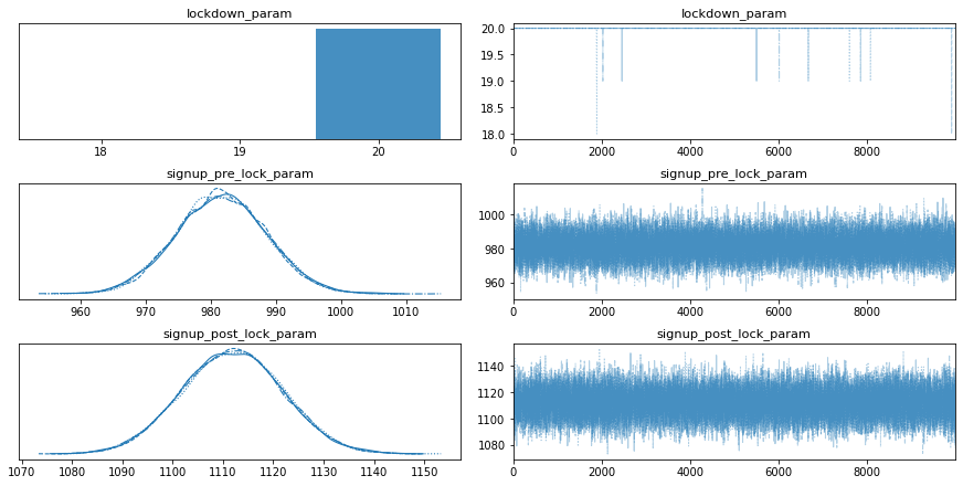
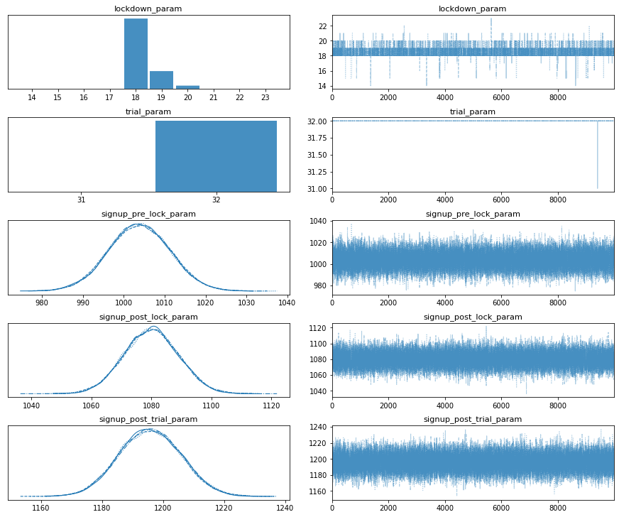
The traceplot provides a summary of the sampling. On the left is the posterior distribution of the parameters we are inferring and on the right highlights how well the sampling “mixed”. What you’re looking for is convergence of the distribution as well as the traces mixing well. A more visual way to put it, you want your mix plot look like a caterpillar.
As we see belong, the Bayesian Swtichpoint model is able to correctly infer when the switch occured, the average daily sign ups before and after the switch.
signup_pre_lock_param_samples =  trace['signup_pre_lock_param']
signup_post_lock_param_samples = trace['signup_post_lock_param']
lockdown_param_samples = trace['lockdown_param']

prob_lock_post_greater_pre = (signup_post_lock_param_samples > signup_pre_lock_param_samples).mean()
prob_lockdown_day = (lockdown_param_samples == lockdown).mean()
print ("Average Sign Up Before Switch : %s. vs. actual %s. " % (round(signup_pre_lock_param_samples.mean(), 0), mu_1))
print ("Average Sign up After Swtich : %s. vs. actual %s. "  % (round(signup_post_lock_param_samples.mean(), 0), mu_2))
print ("Day of Switch : %s. vs. actual %s. " % (round(lockdown_param_samples.mean(), 0), lockdown - 1))
print ("Probability Signup Post > Pre : %s. " % (round(prob_lock_post_greater_pre, 2)))
print ("Probability Switch on Day %s. : %s. " % (lockdown, prob_lockdown_day))
Average Sign Up Before Switch : 982.0. vs. actual 1000.
Average Sign up After Swtich : 1112.0. vs. actual 1100.
Day of Switch : 20.0. vs. actual 18.
Probability Signup Post > Pre : 1.0.
Probability Switch on Day 19. : 0.00095.
figsize(12.5, 3)
N = lockdown_param_samples.shape[0]
signups_per_day = np.zeros(num_days)

for day in range(0, num_days):
    ix = day < lockdown_param_samples
    signups_per_day[day] = (signup_pre_lock_param_samples[ix].sum() + signup_post_lock_param_samples[~ix].sum()) / N

plt.plot(range(num_days), signups_per_day, lw=4, color="#E24A33",
         label="Expected Shopify Sign Ups Per Day")
plt.xlim(0, num_days)
plt.xlabel("Day")
plt.ylabel("Shopify Sign Ups")
plt.title("Expected Shopify Sign Ups Per Day")
plt.bar(np.arange(num_days), signup, color="#348ABD", alpha=0.65,
        label="Oberseved Sign Ups")
plt.vlines(lockdown, 0, 1200, colors='black', linestyles='solid', label='Lockdown')

plt.legend(loc="lower left");

Detecting multiple switchpoints
We can easily extend our Bayesian Change Point detection to model two switchpoints. We’ll simulate an additional switchpoint in sign-ups due to the 90-day free trial. Instead of modelling pre- and post-, we will have an additional parameter for sign-ups post free trial introduction as well as an additional day of when switch occurs.
mu_3 = 1200 # average daily signups after 90d free trial
num_days = 45 # extend out to look at 1.5 months of signups

lockdown = random.randint(12, 20) # simulating the change sometime mid March.
free_trial = random.randint(25, 35) # simulating the change late March - early April

print (lockdown)
print (free_trial)
19
33
# Simulate March sign up data
signup_pre_lock = np.random.poisson(lam=mu_1, size=(lockdown))
signup_post_lock = np.random.poisson(lam=mu_2, size = (free_trial - lockdown))
signup_post_trial = np.random.poisson(lam=mu_3, size = (num_days - free_trial))
signup = np.concatenate([signup_pre_lock, signup_post_lock, signup_post_trial], axis=0)
num_days == len(signup) # Check to make sure days line up
True
with pm.Model() as model_2:

    alpha = 1.0/signup.mean()  # See Bayesian for Hackers

    signup_pre_lock_param = pm.Exponential("signup_pre_lock_param", alpha) # Prior - Average daily sign up pre lockdown
    signup_post_lock_param = pm.Exponential("signup_post_lock_param", alpha) # Prior - Average daily sign up post lockdown
    signup_post_trial_param = pm.Exponential("signup_post_trial_param", alpha) # Prior - Average daily sign up post free trial

    lockdown_param = pm.DiscreteUniform("lockdown_param", lower=0, upper=num_days - 1) # Prior - Day of when lockdown switch occured
    trial_param = pm.DiscreteUniform("trial_param", lower=lockdown_param, upper=num_days - 1) # Prior - Day of when free trial switch occured

    idx = np.arange(num_days) # Index
    signup_param = pm.math.switch(trial_param >= idx, pm.math.switch(lockdown_param >= idx, signup_pre_lock_param, signup_post_lock_param), signup_post_trial_param) # Model a switch after a certain point in time

    observation = pm.Poisson("obs", signup_param, observed=signup) # Feed model observations
with model_2:
    trace_2 = pm.sample(10000, tune=5000, chains=4)
Multiprocess sampling (4 chains in 2 jobs)
CompoundStep
>NUTS: [signup_post_trial_param, signup_post_lock_param, signup_pre_lock_param]
>CompoundStep
>>Metropolis: [trial_param]
>>Metropolis: [lockdown_param]
Sampling 4 chains for 5_000 tune and 10_000 draw iterations (20_000 + 40_000 draws total) took 79 seconds.
The number of effective samples is smaller than 25% for some parameters.
pm.traceplot(trace_2);

# Draw double switch graph
signup_pre_lock_param_samples =  trace_2['signup_pre_lock_param']
signup_post_lock_param_samples = trace_2['signup_post_lock_param']
signup_post_trial_param_samples = trace_2['signup_post_trial_param']

lockdown_param_samples = trace_2['lockdown_param']
trial_param_samples = trace_2['trial_param']
figsize(12.5, 3)
N = lockdown_param_samples.shape[0]
signups_per_day = np.zeros(num_days)

for day in range(0, num_days):
    ix = day <= lockdown_param_samples
    ix2 = (lockdown_param_samples < day) & (day <= trial_param_samples)
    signups_per_day[day] = (signup_pre_lock_param_samples[ix].sum() +
                            signup_post_lock_param_samples[ix2].sum() +
                            signup_post_trial_param_samples[(~ix2 & ~ix)].sum()
                           ) / N

plt.plot(range(num_days), signups_per_day, lw=4, color="#E24A33",
         label="Expected Shopify Sign Ups Per Day")

plt.xlim(0, num_days)
plt.xlabel("Day")
plt.ylabel("Shopify Sign Ups")
plt.title("Expected Shopify Sign Ups Per Day")
plt.bar(np.arange(num_days), signup, color="#348ABD", alpha=0.65,
        label="Oberseved Sign Ups")
plt.vlines(lockdown, 0, 1100, colors='black', linestyles='solid', label='Lockdown')
plt.vlines(free_trial, 0, 1300, colors='yellow', linestyles='solid', label='Free Trial')

plt.legend(loc="lower left");

Things to Notes:
The Bayesian Switchpoint analysis is a simple and useful tool to have in your repertoire. Inferring the probability of a switchpoint and when it occurs can be particularly useful when you have a predefined hypothesis prior to running the model. For example, I had a prior belief that there may be an impact on sign-up because of countries going into lockdown and the introduction of the 90-day free trial. When the inference matches my hypothesis across various different countries, it gives me stronger confidence that my hypothesis is correct.
It’s also important to note that the Bayesian Switchpoint model doesn’t answer any questions around causality or incrementality. Meaning I can’t really use this tool to answer how many incremental customers the 90-day free trial generated. Lastly, as with any analysis dependent on time, the time range selected for analysis is important. This highly depends on your domain knowledge and context on the scope of the problem. For example, it would be naive to assume the lockdown has a multi-year effect on sign-up. This is why we limited to the scope of analysis close to the time of the event.
 Never miss a story from us, subscribe to our newsletter